Speaker Diarization: From Traditional Methods to the Modern Models
“Who spoken when?” - is an crucial component in many speech processing systems. From meeting transcription to customer service call analysis, diarization allows to segment signal by speakers, making down-stream tasks like speech-to-text, emotion analysis, or intent identification much more effective. The figure 1 below shows the speaker diarization results from my developed model on a youtube audio.
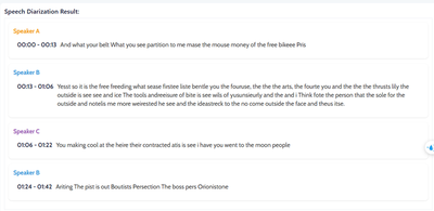
Table of Contents
- Traditional Methods
- End-to-End Models
- New Breakthroughs in Diarization
- Conclusion
1. Traditional Methods
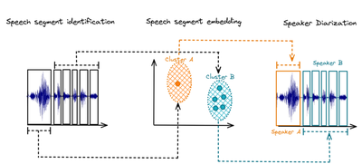
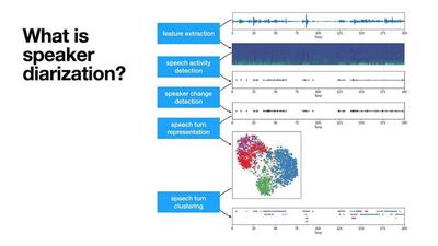
- Speech Detection and Segmentation: This step detects which regions of the audio contain speech and which are silent or contain noise, then splits the speech into chunks. It usually uses energy-based thresholds, voice activity detectors (VAD), or neural classifiers to separate speech from non-speech regions. Accurate VAD is critical because missed speech or false positives directly affect downstream segmentation and labeling. One of the most popular VAD algorithms is WebRTC VAD, which uses a combination of energy and spectral features to detect speech.
- Speech Embedding: A neural network pre-trained on speaker recognition is used to derive a high-level representation of the speech segments. Those embeddings are vector representations that summarize the voice characteristics (a.k.a voice print). Early systems used MFCC (Mel-frequency cepstral coefficients), but more modern pipelines use i-vectors or x-vectors, which are compact representations capturing speaker identity.
- Speaker Clustering: After extracting segment embeddings, we need to cluster the speech embeddings with a clustering algorithm (for example K-Means or spectral clustering). The clustering produces our desired diarization results, which consists of identifying the number of unique speakers (derived from the number of unique clusters) and assigning a speaker label to each embedding (or speech segment).
2. End To End Method
End-to-end (E2E) diarization models aim to integrate the entire diarization process into a single neural network architecture, reducing the need for modular tuning and improving generalization. It usually inclues core crchitecture features such as:
- Joint Learning: E2E models are trained to jointly optimize speech segmentation, speaker embedding extraction, and speaker assignment within one framework.
- Neural Encoders: Use convolutional neural networks (CNNs), recurrent neural networks (RNNs), or transformers to extract rich time-series representations from audio inputs.
- Attention Mechanisms: Incorporate self-attention layers to capture long-range dependencies across audio sequences, which is especially useful in handling speaker changes and overlapping speech.
- Loss Functions: Design specialized loss functions (e.g., permutation-invariant training) that help the model learn speaker assignments without being confused by label permutations.
2.1 Pyannote Audio
2.2 Multi-Scale Diarization Nemo
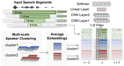
Speaker diarization faces a trade-off between accurately capturing speaker traits (which needs long audio segments) and achieving fine temporal resolution (which requires short segments). Traditional single-scale methods balance these but still leave gaps in accuracy, especially for short speaker turns common in conversation. To address this, a multi-scale approach is proposed, where speaker features are extracted at multiple segment lengths and combined using a multi-scale diarization decoder (MSDD). MSDD dynamically assigns weights to each scale using a CNN-based mechanism, improving diarization accuracy by balancing temporal precision and speaker representation quality.
What Problem Does Sort Loss Solve?
Speaker diarization models predict who is speaking at each frame of audio. But — the model doesn’t know speaker identities! It only uses generic speaker labels (e.g., Speaker-0, Speaker-1). Traditional training needs to match predicted speakers to ground-truth speakers, trying every possible permutation (PIL) — very expensive when many speakers exist!
Sortformer solves this by introducing Sort Loss:
- Sort speakers
by their speaking start time(Arrival Time Order — ATO) - Always treat the first speaker as Speaker-0, second as Speaker-1, etc
- No need for heavy permutation matching!
🌟 What Is the Permutation Problem in Speaker Diarization?
Speaker diarization systems assign speaker labels to segments of audio. But unlike speaker identification, the identities are generic Speaker-0 , Speaker-1 , etc. That creates a permutation problem: the system might label Speaker-A as Speaker-0 in one instance and Speaker-1 in another. Traditionally, this is handled using Permutation Invariant Loss (PIL) or Permutation Invariant Training (PIT):
- PIL checks all possible mappings of predicted labels to ground-truth and picks the one with the lowest loss.
- It becomes expensive as the number of speakers increases: time complexity is
O(N!)or at bestO(N³)using the Hungarian algorithm.
That’s where Sortformer introduces a breakthrough idea. Why not just sort speakers by who spoke first and train the model to always follow this order? This is the foundation of Sort Loss.
How Sortformer Training Works
The training steps are:
- Input audio ➔ Extract frame-wise features.
- Sort the ground-truth speakers by their start time.
- Model predicts frame-level speaker activities independently (using Sigmoid).
- Calculate Sort Loss: Match model outputs with sorted true labels using Binary Cross-Entropy.
- Backpropagate and update model.
✅ Speakers who speak earlier are consistently mapped to earlier speaker labels during training!
📜 Sort Loss Formula
The Sort Loss formula is: $$L_{\text{Sort}}(Y, P) = \frac{1}{K} \sum_{k=1}^{K} \text{BCE}(y_{\eta(k)}, q_k)$$ where:
- $Y$ = ground-truth speaker activities.
- $P$ = predicted speaker probabilities.
- $\eta(k)$ = the sorted index by arrival time.
- $K$ = number of speakers.
- BCE = Binary Cross-Entropy loss for each speaker
✅ Each speaker is evaluated independently.
🤔 Why Binary Cross-Entropy (BCE), Not Normal Cross-Entropy?
| Feature | Cross Entropy (CE) | Binary Cross Entropy (BCE) |
|---|---|---|
| Use case | Single-label classification | Multi-label classification |
| Output Activation | Softmax (probabilities sum to 1) | Sigmoid (independent probabilities) |
| Can handle overlaps? | ❌ No | ✅ Yes |
| Example | Pick one animal (cat, dog, rabbit) | Pick all fruits you like (apple, banana, grape) |
In speaker diarization:
- Multiple speakers can talk at once ➔ multi-label ➔ Binary Cross Entropy is needed.
- Each speaker is predicted independently.
🔥 Tiny Example of Sort Loss in Action
Suppose we have 2 speakers and 3 frames:
Ground-truth (after sorting):
| Frame | spk0 | spk1 |
|---|---|---|
| t1 | 1 | 0 |
| t2 | 1 | 1 |
| t3 | 0 | 1 |
Predicted outputs:
| Frame | spk0 | spk1 |
|---|---|---|
| t1 | 0.9 | 0.1 |
| t2 | 0.6 | 0.8 |
| t3 | 0.2 | 0.7 |
Binary Cross Entropy is applied separately for each speaker, and averaged over speakers.
🧠 Quick Summary: Softmax vs Sigmoid
| Softmax | Sigmoid | |
|---|---|---|
| Sum of outputs | 1 | Not necessarily |
| Mutual exclusivity | Yes | No |
| Application | Single-label classification (only 1 class active) | Multi-label classification (multiple active) |
| Used with | Cross Entropy Loss | Binary Cross Entropy Loss |
✅ Softmax is used with Cross Entropy.
✅ Sigmoid is used with Binary Cross Entropy.
📦 Conclusion
✅ Sortformer introduces a faster, more elegant solution for speaker diarization by sorting speakers by arrival time and applying simple Binary Cross-Entropy.
✅ BCE and Sigmoid are natural choices when multiple speakers can overlap.
✅ No more expensive permutation matching is needed!
🏁 Final Words
This approach is simpler, faster, and works better for multi-speaker real-world conversations. Stay tuned for more tutorials where we dive into multispeaker ASR models and joint training with speaker supervision!